Visualizations
Many Stats Can Be Plotted via Plot Recipes
s = fit!(Series(Hist(25), Hist(-5:5)), randn(10^6))
plot(s)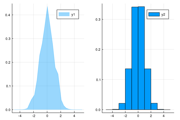
Naive Bayes Classifier
The NBClassifier type stores conditional histograms of the predictor variables, allowing you to plot approximate "group by" distributions:
# make data
x = randn(10^5, 5)
y = x * [1,3,5,7,9] .> 0

o = NBClassifier(5, Bool)  # 5 predictors with Boolean categories
fit!(o, (x, y))
plot(o)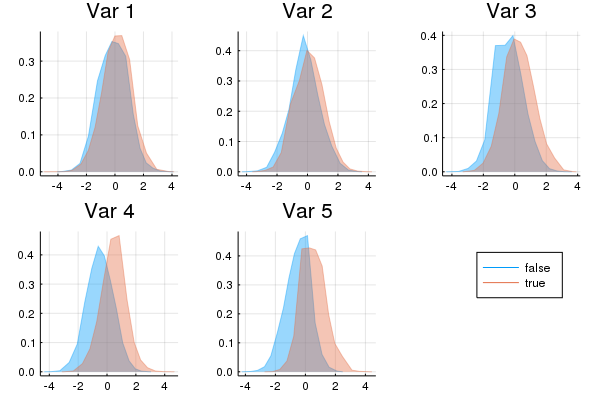
Mosaic Plots
The Mosaic type allows you to plot the relationship between two categorical variables. It is typically more useful than a bar plot, as class probabilities are given by the horizontal widths.
x = rand([true, true, false], 10^5)
y = map(xi -> xi ? rand(1:3) : rand(1:4), x)
o = fit!(Mosaic(Bool, Int), [x y])
plot(o)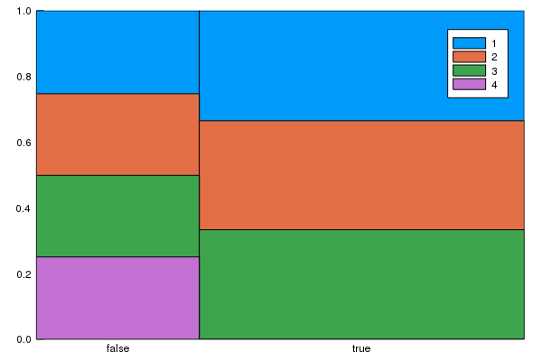
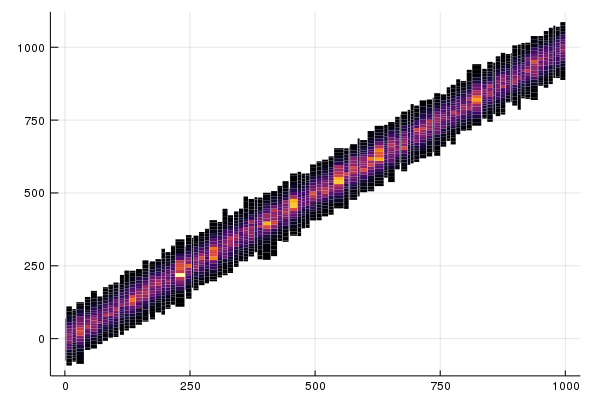
Partitions
The Partition type summarizes sections of a data stream using any OnlineStat, and is therefore extremely useful in visualizing huge datasets, as summaries are plotted rather than every single observation.
Continuous Data
y = cumsum(randn(10^6)) + 100randn(10^6)

o = Partition(Hist(10))

fit!(o, y)

plot(o, xlab = "Nobs")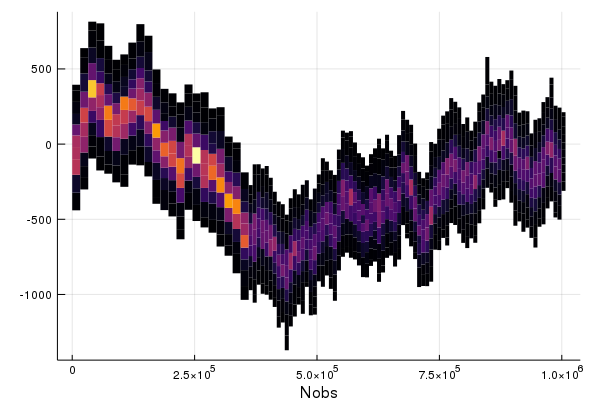
o = Partition(Mean())
o2 = Partition(Extrema())

s = Series(o, o2)

fit!(s, y)

plot(s, layout = 1, xlab = "Nobs")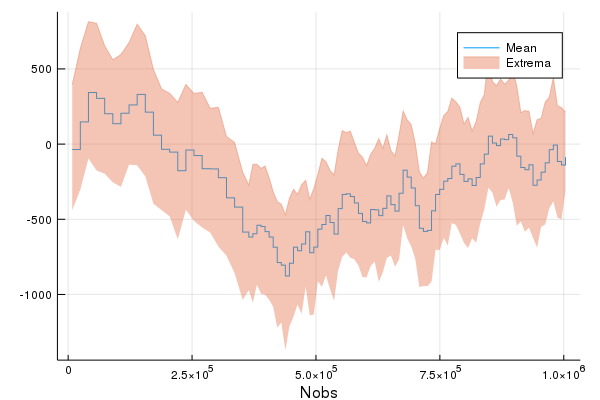
Plot a custom function of the OnlineStats (default is value)
Plot of mean +/- standard deviation:
o = Partition(Variance())

fit!(o, y)

plot(o, x -> [mean(x) - std(x), mean(x), mean(x) + std(x)], xlab = "Nobs")
savefig("partition_ci.png"); nothing # hide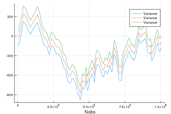
Categorical Data
y = rand(["a", "a", "b", "c"], 10^6)

o = Partition(CountMap(String), 75)

fit!(o, y)

plot(o, xlab = "Nobs")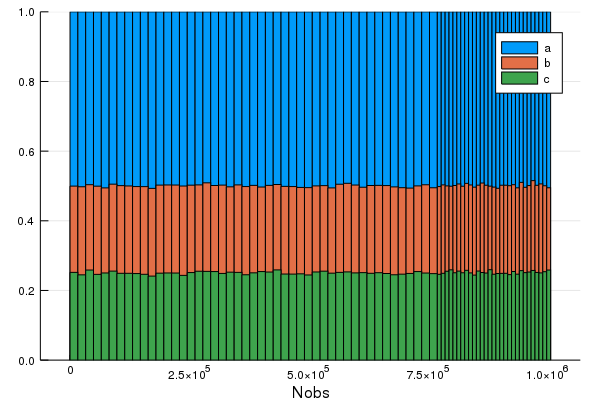
Indexed Partitions
The Partition type can only track the number of observations in the x-axis. If you wish to plot one variable against another, you can use an IndexedPartition.
x = randn(10^5)
y = x + randn(10^5)

o = fit!(IndexedPartition(Float64, Hist(10)), [x y])

plot(o, ylab = "Y", xlab = "X")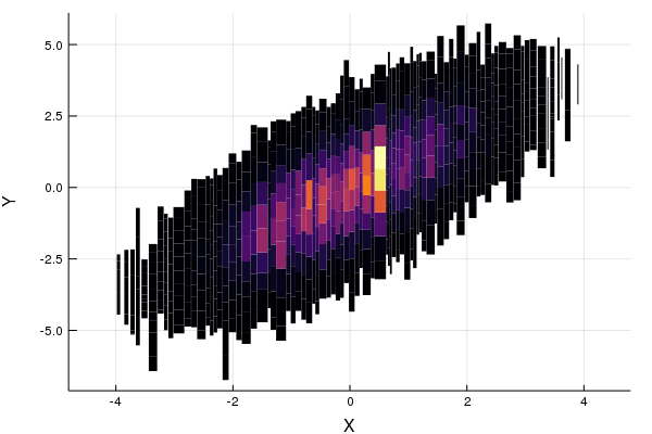
x = rand('a':'z', 10^5)
y = Float64.(x) + randn(10^5)

o = fit!(IndexedPartition(Char, Extrema()), [x y])

plot(o, xlab = "Category")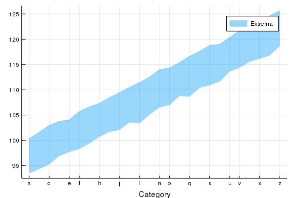
x = rand(10^5)
y = rand(1:5, 10^5)

o = fit!(IndexedPartition(Float64, CountMap(Int)), zip(x,y))

plot(o, xlab = "X", ylab = "Y")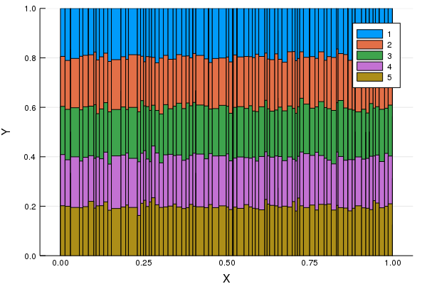
x = rand(1:1000, 10^5)
y = x .+ 30randn(10^5)

o = fit!(IndexedPartition(Int, Hist(20)), zip(x,y))

plot(o)