Weights

Many OnlineStats are parameterized by a Weight that controls the influence of new observations. If the OnlineStat is capable of calculating the same result as a corresponding offline estimator, it will have a keyword argument weight. If the OnlineStat uses stochastic approximation, it will have a keyword argument rate (see this great resource on stochastic approximation algorithms).

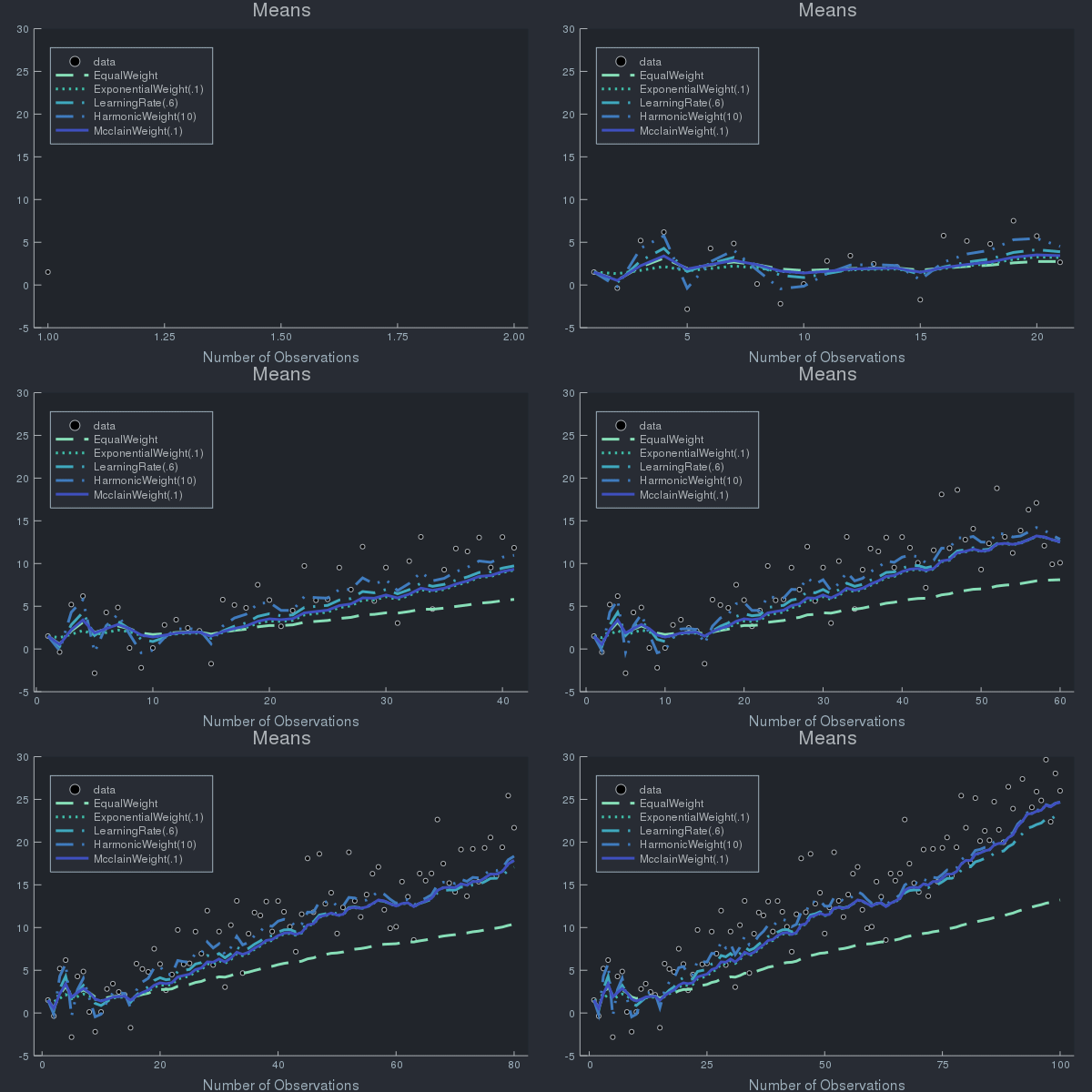
Consider how weights affect the influence of the next observation on an online mean $\theta^{(t)}$, as many OnlineStats use updates of this form. A larger weight $\gamma_t$ puts higher influence on the new observation $x_t$:

\[\theta^{(t)} = (1-\gamma_t)\theta^{(t-1)} + \gamma_t x_t\]

Note

The values produced by a Weight must follow two rules:

$\gamma_1 = 1$ (guarantees $\theta^{(1)} = x_1$)
$\gamma_t \in (0, 1), \quad \forall t > 1$ (guarantees $\theta^{(t)}$ stays inside a convex space)

Info

The notion of weighting in OnlineStats is fundamentally different than StatsBase.AbstractWeights.

In OnlineStats, a weight determines the influence of an observation compared to the current state of the statistic.
In StatsBase, a weight determines the influence of an observation in the overall calculation of the statistic.

julia> using OnlineStats, StatsBase
julia> x = 1:99;
julia> w = fill(0.1, 99);
       
       # StatsBase: All weights == 0.1
julia> mean(x) ≈ mean(x, aweights(w)) ≈ mean(x, fweights(w)) ≈ mean(x, pweights(w))
       
       # OnlineStats: All weights == 0.1true
julia> o = fit!(Mean(weight = n -> 0.1), x)Mean: n=99 | value=90.0003
julia> mean(x)  # Every observation has equal influence over statistic.50.0
julia> value(o)  # Recent observations have higher influence over statistic.90.00026561398887

Weight Types

OnlineStatsBase.EqualWeight — Type

EqualWeight()

Equally weighted observations.

$γ(t) = 1 / t$

source

OnlineStatsBase.ExponentialWeight — Type

ExponentialWeight(λ::Float64)
ExponentialWeight(lookback::Int)

Exponentially weighted observations. Each weight is λ = 2 / (lookback + 1).

ExponentialWeight does not satisfy the usual assumption that γ(1) == 1. Therefore, some statistics have an implicit starting value.

# E.g. Mean has an implicit starting value of 0.
o = Mean(weight=ExponentialWeight(.1))
fit!(o, 10)
value(o) == 1

$γ(t) = λ$

source

OnlineStatsBase.LearningRate — Type

LearningRate(r = .6)

Slowly decreasing weight. Satisfies the standard stochastic approximation assumption $∑ γ(t) = ∞, ∑ γ(t)^2 < ∞$ if $r ∈ (.5, 1]$.

$γ(t) = inv(t ^ r)$

source

OnlineStatsBase.LearningRate2 — Type

LearningRate2(c = .5)

Slowly decreasing weight.

$γ(t) = inv(1 + c * (t - 1))$

source

OnlineStatsBase.HarmonicWeight — Type

HarmonicWeight(a = 10.0)

Weight determined by harmonic series.

$γ(t) = a / (a + t - 1)$

source

OnlineStatsBase.McclainWeight — Type

McclainWeight(α = .1)

Weight which decreases into a constant.

$γ(t) = γ(t-1) / (1 + γ(t-1) - α)$

source

Custom Weighting

The Weight can be any callable object that receives the number of observations as its argument. For example:

weight = inv will have the same result as weight = EqualWeight().
weight = x -> .01 will have the same result as weight = ExponentialWeight(.01)

julia> y = randn(100);
julia> fit!(Mean(weight = EqualWeight()), y)Mean: n=100 | value=-0.0360879
julia> fit!(Mean(weight = inv), y)Mean: n=100 | value=-0.0360879

Weights

Weight Types

Custom Weighting

Example of Weight Effects using Data with Concept Drift